What is Spark?
What is Spark?
Yesterday I completed the Data Camp Introduction to Sparklyr course. This covered an introduction to Spark, as well as sparklyr, a package to interface with spark through R. Before I forget it all, I wanted to write down an explanation of it, some key points and functions.
Spark is an open source cluster-computer framework, maintained by the Apache Software Foundation. If like me, that doesn’t help much, then this is a more simplified explanation/motivation for it.
Suppose you want to analyse a dataset of your personal taxi (or uber) journeys. Unless you work as a taxi driver (or for uber), you probably won’t have many. You’ve got a bit of expierence with R, so you load it into R Studio and carry on. Simple!
But now, let’s say you need to analyse the Uber Journeys for everyone in London. This is a lot more data. R is limited by the size of RAM on your computer. If the size of the data you wish to process is bigger than the size of your RAM, then your out of luck. If it’s even approaching the limit, it will probably be quite slow.
What do you do? Well there are many options. An obvious one is to get a faster computer, with more RAM. Spark is an alternative solution. Instead of one powerful computer, it provides a framework to let you create and utilise a “cluster” of many computers to do your data analysis bidding. This is a simplification of all the benefits provided, but it helps to provide a simple motivation.
Unfortunately for R users out there, Spark is written in Scala. Until recently to work with it, you’ve needed to use Scala, Java or Python. sparklyr is the R interface to Spark. With it, you can work with Spark with familiar dplyr methods.
There are a few differences to understand when using splarklyr to manipulate data in the spark cluster rather than dplyr on your local machine
Examples
library(sparklyr)
library(dplyr)
## Warning: package 'dplyr' was built under R version 3.3.3##
## Attaching package: 'dplyr'## The following objects are masked from 'package:stats':
##
## filter, lag## The following objects are masked from 'package:base':
##
## intersect, setdiff, setequal, unionlibrary(ggplot2)## Warning: package 'ggplot2' was built under R version 3.3.3# spark_install()
sc <- spark_connect("local") # connect to my local spark cluster (of one computer)## * Using Spark: 2.1.0Explanation of CopyTo
In Spark, the data is stored on the cluster. If the data you wish to analyse is on your local machine, then you will need to copy it to your Spark cluster. You can do this with dplyr::copy_to() (or sparklyr::sdf_copy_to()). This creates an object on your spark cluster. The variable you assign this will not be a dataframe, but a reference to the Spark Dataframe on the cluster.
diamonds_sc <- dplyr::copy_to(sc,diamonds, overwrite = T)


class(diamonds_sc)
## [1] "tbl_spark" "tbl_sql" "tbl_lazy" "tbl"str(diamonds_sc)## List of 2
## $ src:List of 1
## ..$ con:List of 10
## .. ..$ master : chr "local[4]"
## .. ..$ method : chr "shell"
## .. ..$ app_name : chr "sparklyr"
## .. ..$ config :List of 5
## .. .. ..$ sparklyr.cores.local : int 4
## .. .. ..$ spark.sql.shuffle.partitions.local: int 4
## .. .. ..$ spark.env.SPARK_LOCAL_IP.local : chr "127.0.0.1"
## .. .. ..$ sparklyr.csv.embedded : chr "^1.*"
## .. .. ..$ sparklyr.shell.driver-class-path : chr ""
## .. .. ..- attr(*, "config")= chr "default"
## .. .. ..- attr(*, "file")= chr "C:\\Users\\IBM_ADMIN\\Documents\\R\\win-library\\3.3\\sparklyr\\conf\\config-template.yml"
## .. ..$ spark_home : chr "C:\\Users\\IBM_ADMIN\\AppData\\Local\\spark\\spark-2.1.0-bin-hadoop2.7"
## .. ..$ backend :Classes 'sockconn', 'connection' atomic [1:1] 6
## .. .. .. ..- attr(*, "conn_id")=<externalptr>
## .. ..$ monitor :Classes 'sockconn', 'connection' atomic [1:1] 5
## .. .. .. ..- attr(*, "conn_id")=<externalptr>
## .. ..$ output_file : chr "C:\\Users\\IBM_AD~1\\AppData\\Local\\Temp\\RtmpYvXYE4\\file22dc5e2c5243_spark.log"
## .. ..$ spark_context:Classes 'spark_jobj', 'shell_jobj' <environment: 0x000000000b8a7880>
## .. ..$ java_context :Classes 'spark_jobj', 'shell_jobj' <environment: 0x000000000a96d050>
## .. ..- attr(*, "class")= chr [1:3] "spark_connection" "spark_shell_connection" "DBIConnection"
## ..- attr(*, "class")= chr [1:3] "src_spark" "src_sql" "src"
## $ ops:List of 2
## ..$ x :Classes 'ident', 'character' chr "diamonds"
## ..$ vars: chr [1:10] "carat" "cut" "color" "clarity" ...
## ..- attr(*, "class")= chr [1:3] "op_base_remote" "op_base" "op"
## - attr(*, "class")= chr [1:4] "tbl_spark" "tbl_sql" "tbl_lazy" "tbl"glimpse(diamonds_sc)## Observations: 25
## Variables: 10
## $ carat <dbl> 0.23, 0.21, 0.23, 0.29, 0.31, 0.24, 0.24, 0.26, 0.22, ...
## $ cut <chr> "Ideal", "Premium", "Good", "Premium", "Good", "Very G...
## $ color <chr> "E", "E", "E", "I", "J", "J", "I", "H", "E", "H", "J",...
## $ clarity <chr> "SI2", "SI1", "VS1", "VS2", "SI2", "VVS2", "VVS1", "SI...
## $ depth <dbl> 61.5, 59.8, 56.9, 62.4, 63.3, 62.8, 62.3, 61.9, 65.1, ...
## $ table <dbl> 55, 61, 65, 58, 58, 57, 57, 55, 61, 61, 55, 56, 61, 54...
## $ price <int> 326, 326, 327, 334, 335, 336, 336, 337, 337, 338, 339,...
## $ x <dbl> 3.95, 3.89, 4.05, 4.20, 4.34, 3.94, 3.95, 4.07, 3.87, ...
## $ y <dbl> 3.98, 3.84, 4.07, 4.23, 4.35, 3.96, 3.98, 4.11, 3.78, ...
## $ z <dbl> 2.43, 2.31, 2.31, 2.63, 2.75, 2.48, 2.47, 2.53, 2.49, ...Explanation of Collect
Spark uses lazy evaluation. Commands sent to it will not be evaluated until needed. All of this is done on the cluster. What you recieve back from the cluster can be thought of as just a snapshot of the data’s results, not the data itself. Say you wished to use the data to create a plot, you would need to bring it back to your local R session. This is done with the dplyr::collect() function
# Notice what is returned.
diamonds_sc %>%
  group_by(color) %>%
  summarise(mean_price = mean(price)) %>%
  arrange(desc(mean_price)) %>%
  str()
## List of 2
## $ src:List of 1
## ..$ con:List of 10
## .. ..$ master : chr "local[4]"
## .. ..$ method : chr "shell"
## .. ..$ app_name : chr "sparklyr"
## .. ..$ config :List of 5
## .. .. ..$ sparklyr.cores.local : int 4
## .. .. ..$ spark.sql.shuffle.partitions.local: int 4
## .. .. ..$ spark.env.SPARK_LOCAL_IP.local : chr "127.0.0.1"
## .. .. ..$ sparklyr.csv.embedded : chr "^1.*"
## .. .. ..$ sparklyr.shell.driver-class-path : chr ""
## .. .. ..- attr(*, "config")= chr "default"
## .. .. ..- attr(*, "file")= chr "C:\\Users\\IBM_ADMIN\\Documents\\R\\win-library\\3.3\\sparklyr\\conf\\config-template.yml"
## .. ..$ spark_home : chr "C:\\Users\\IBM_ADMIN\\AppData\\Local\\spark\\spark-2.1.0-bin-hadoop2.7"
## .. ..$ backend :Classes 'sockconn', 'connection' atomic [1:1] 6
## .. .. .. ..- attr(*, "conn_id")=<externalptr>
## .. ..$ monitor :Classes 'sockconn', 'connection' atomic [1:1] 5
## .. .. .. ..- attr(*, "conn_id")=<externalptr>
## .. ..$ output_file : chr "C:\\Users\\IBM_AD~1\\AppData\\Local\\Temp\\RtmpYvXYE4\\file22dc5e2c5243_spark.log"
## .. ..$ spark_context:Classes 'spark_jobj', 'shell_jobj' <environment: 0x000000000b8a7880>
## .. ..$ java_context :Classes 'spark_jobj', 'shell_jobj' <environment: 0x000000000a96d050>
## .. ..- attr(*, "class")= chr [1:3] "spark_connection" "spark_shell_connection" "DBIConnection"
## ..- attr(*, "class")= chr [1:3] "src_spark" "src_sql" "src"
## $ ops:List of 4
## ..$ name: chr "arrange"
## ..$ x :List of 4
## .. ..$ name: chr "summarise"
## .. ..$ x :List of 4
## .. .. ..$ name: chr "group_by"
## .. .. ..$ x :List of 2
## .. .. .. ..$ x :Classes 'ident', 'character' chr "diamonds"
## .. .. .. ..$ vars: chr [1:10] "carat" "cut" "color" "clarity" ...
## .. .. .. ..- attr(*, "class")= chr [1:3] "op_base_remote" "op_base" "op"
## .. .. ..$ dots:List of 1
## .. .. .. ..$ color: symbol color
## .. .. ..$ args:List of 1
## .. .. .. ..$ add: logi FALSE
## .. .. ..- attr(*, "class")= chr [1:3] "op_group_by" "op_single" "op"
## .. ..$ dots:List of 1
## .. .. ..$ mean_price:<quosure: local 000000000A0E9570>
## ~mean(price)
## .. .. ..- attr(*, "class")= chr "quosures"
## .. ..$ args: list()
## .. ..- attr(*, "class")= chr [1:3] "op_summarise" "op_single" "op"
## ..$ dots:List of 1
## .. ..$ :<quosure: local 000000000820FF50>
## ~desc(mean_price)
## ..$ args: list()
## ..- attr(*, "class")= chr [1:3] "op_arrange" "op_single" "op"
## - attr(*, "class")= chr [1:4] "tbl_spark" "tbl_sql" "tbl_lazy" "tbl"# To get the actual data we need to use collect! Notice we need to assign it a variable (or pass it directly to ggplot). THe key is to use collect to get the actual data, not the reference to it.
computed_diamonds <- diamonds_sc %>%
group_by(color) %>%
summarise(mean_price = mean(price)) %>%
arrange(desc(mean_price)) %>%
collect()
ggplot(computed_diamonds, aes(color, mean_price)) + geom_bar(stat = 'identity')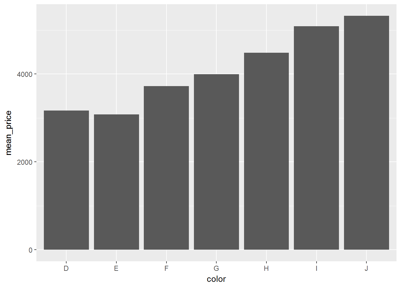
Explanation of Compute
When we run a command in Spark, it is lazily evaluated (see above). The results returned are a reference to the spark cluster, not actual results. As such, if you wish to create an intermediatry table in Spark, you must use the sparklyr::compute() function. This stores thetable in Spark with the data you’ve piped in to it.
diamonds_sc %>%
  group_by(clarity) %>%
  summarise(mean_x = mean(x), mean_y = mean(y), mean_z = mean(z)) %>%
  compute(sc, name = "diamond_size_summary")
## # Source: table<diamond_size_summary> [?? x 4]
## # Database: spark_connection
## clarity mean_x mean_y mean_z
## <chr> <dbl> <dbl> <dbl>
## 1 VVS2 5.218454 5.232118 3.221465
## 2 VVS1 4.960364 4.975075 3.061294
## 3 VS2 5.657709 5.658859 3.491478
## 4 I1 6.761093 6.709379 4.207908
## 5 IF 4.968402 4.989827 3.061659
## 6 SI2 6.401370 6.397826 3.948478
## 7 SI1 5.888383 5.888256 3.639845
## 8 VS1 5.572178 5.581828 3.441007size_summary <- tbl(sc, "diamond_size_summary")
glimpse(size_summary)## Observations: 8
## Variables: 4
## $ clarity <chr> "VVS2", "VVS1", "VS2", "I1", "IF", "SI2", "SI1", "VS1"
## $ mean_x <dbl> 5.218454, 4.960364, 5.657709, 6.761093, 4.968402, 6.40...
## $ mean_y <dbl> 5.232118, 4.975075, 5.658859, 6.709379, 4.989827, 6.39...
## $ mean_z <dbl> 3.221465, 3.061294, 3.491478, 4.207908, 3.061659, 3.94...